
Get ready to put your Excel skills to the test! Brace yourself for a challenge like no other as you dive into the world of spreadsheets. Are you prepared to excel? Let’s find out.
You will use the following functions and features to find answer to four questions:
- Conditional formatting
- COUNTIF
- INDEX
- MATCH
- MAX
- SUM
- SUMIFS
- UNIQUE
Disclaimer
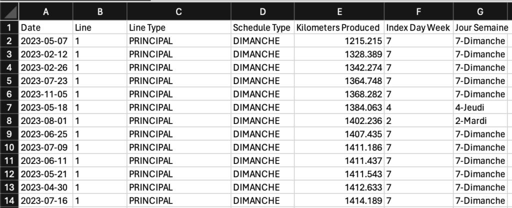
The dataset used in this test belongs to tpg, the public transport operator for the city and canton of Geneva in Switzerland. The dataset has not been modified and is a real world full dataset of Kilometers produced per day per line in 2023 by tpg vehicles (28,606 rows). Latest modification by tpg: 12/02/2024 14:56.
Click here to download the dataset. Below is the preview of the dataset.
Questions
- Highlight the 5 highest kilometers produced.
- Which line travelled the greatest distance in 2023?
- How many line(s) have never travelled during holidays in 2023?
- Is the following statement correct : “In 2023, the tpg vehicles have travelled a distance equivalent to 728 times around the Earth” ?
Answers
1. Here are the steps to take to highlight the 5 highest kilometers produced:
- Select all values under the column Killometers Produced by selecting the first value (cell E2) and then hiting Ctrl + Shift + Down arrow
- Select Conditional Formatting under the Home tab
- Select Top/Bottom Rules then Top 10 Items…
- Now replace 10 by 5 and hit OK. That’s it.
- To see the highlighted values, you can sort the Kilometers Produced column in descending order.
2. The line 14 is the line which travelled the greatest distance in 2023.
Here is how to proceed:
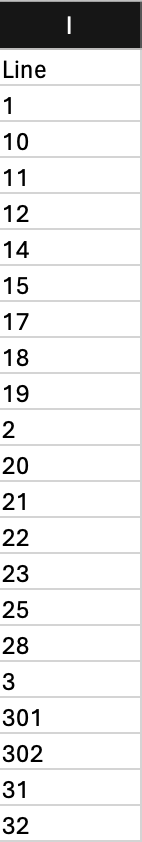
- First of all let’s use UNIQUE function to extract all individual lines. The result of this step is an array. We assign it a column named Line.
=UNIQUE(B2:B28607)The result looks like this (sample):
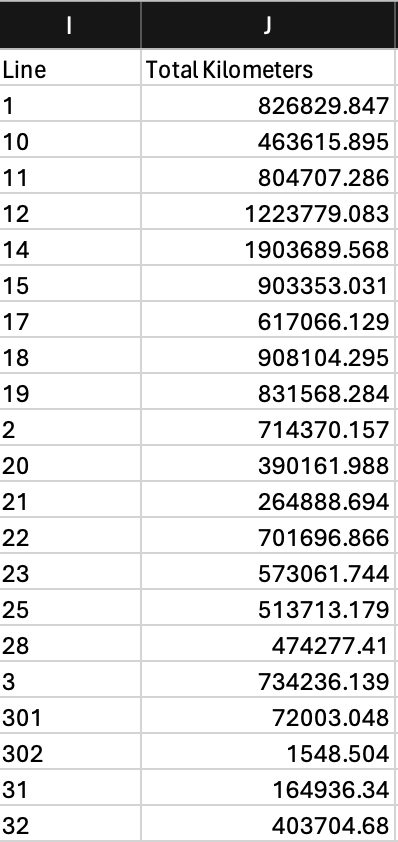
- Secondly let’s use SUMIFS function to find the total kilometers produced by each line. We assign the result to a column named Total Kilometers. Learn more about SUMIFS function here.
=SUMIFS($E$2:$E$28607,$B$2:$B$28607,I2)The result is something like this (sample):
- Finally let’s use a combinaison of three functions to find the line corresponding to the highest total kilometers produced, the result is the answer to this question. Find below the detailed explanation of the formula.
=INDEX(I2#,MATCH(MAX(J2:J108),J2:J108,0))INDEX, this function take an array I2# and a row number MATCH(MAX(J2:J108),J2:J108,0)(column number too but optional) to return a value from the array. The retuned will be the answer of to this question.,
MATCH, we used this function because it is not possible to use VLOOKUP function as the value we are looking for is in the column preceding the column of the known value (of couse we can change the order of columns but we just feel like using MATCH). Here we find the position of the greatest value under the Total Kilometers column. The function takes a lookup value MAX(J2:J108), the array in which to look for J2:J108 and return the postion of the lookup value, which is the row number for INDEX function.
MAX, this function find the greatest value in the Total Kilometers column, It takes the range of values J2:J108 and returns the maximum value, which is the lookup value for MATCH function.
If we write the formula correctly, we will get 14 which means that among the lines of tpg, the line 14 is the line which travelled the greatest distance in 2023.
3- 10 lines have never travelled during holidays in 2023.
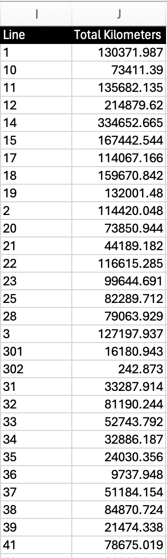
- Using the Line column we have obtained through the function UNIQUE above, we can apply the SUMIFS formula below to find the total kilometers produced by each Line during holydays. For that the Schedule Type must be equals to VACANCES (which means holidays in french). We assign the result to a column named Total Kilometers.
=SUMIFS($E$2:$E$28607,$B$2:$B$28607,I2,$D$2:$D$28607,"VACANCES")In the formula above you can notice that we have two couples of criteria_range, criteria ($B$2:$B$28607,I2 and $D$2:$D$28607,”VACANCES”). Refer to this tutorial to learn more on SUMIFS.
If it is done correctly the result will be the following (sample):
- Now that we have the above data, knowing that when the Total Kilometers of a line is 0, it means that the line has not travelled, we can use COUNTIF function to count the values under the Total Kilometers which are equals to 0, which means we are indirectly counting the lines which have not travelled during VACANCES (holydays). The COUNTIF function takes a range and a creteria. If a value in the range satisfies the criteria it count 1, if another one satisfies it counts 2, and so on.
=COUNTIF(J2:J108,0)The result is 9, which means that 9 lines of tpg have not travelled during holidays in 2023.
4- The statement is true because when we some all the values under Kilometers Produced column and divide it by the circumference of earth we get 728.
Here is how we do that:
- First, use SUM function to some all values of the column Kilometers Produced from the original dataset. Here is the formula:
=SUM(E2:E28607)The result is 29179163.89
- Next, divide the result by the circumference of earth (40075 km) and you get a number close to 728.
Shout-out to tpg for making their data public.
SOME BOOKS TO LEARN EXCEL
- Excel All-in-One For Dummies
- Excel Made Easy: The Ultimate Crash Course to Master Excel Without Getting Overwhelmed
- Excel Basics In 30 Minutes: The beginner’s guide to Microsoft Excel, Excel Online, and Google Sheets
As an Amazon Associate, I earn from qualifying purchases.